A 2D Pathfinder written in C++ using the stb_image library for image rendering. The pathfinder utlizes the A* algorithm to find the optimal path.
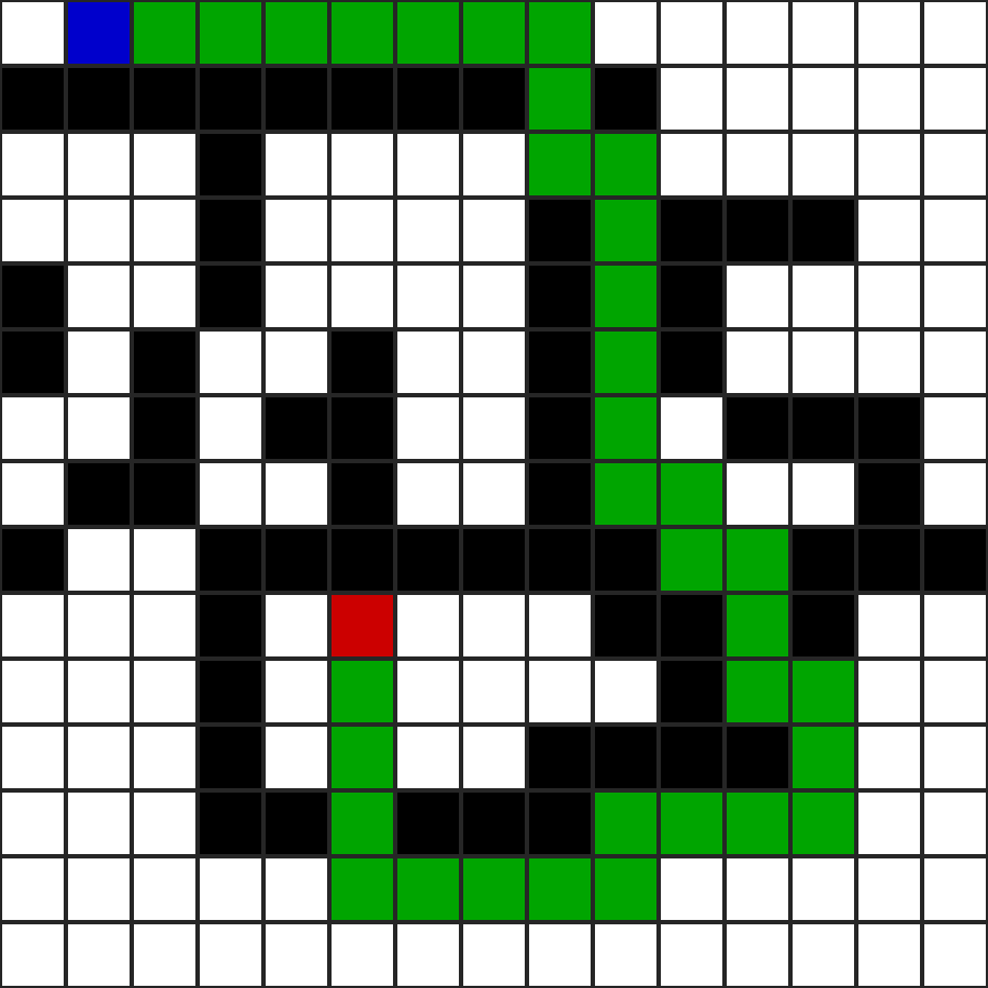
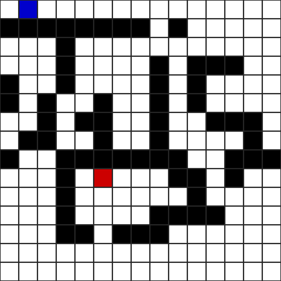
The pathfinder needs to be given a map, starting and ending point along with some configuration. Based on this data, it will output a map along with the solution.


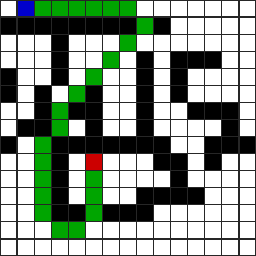
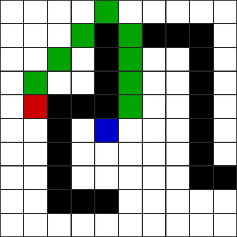
If we change the ending node, a new optimal path will be calculated and shown in the output image.

Specifications of the pathfinder:-
// The Grid State
...
int gridState[NUMBER_ROWS * NUMBER_COLUMNS] = {0, 2, 0, 0, 0, 0, 0, 0, 0, 0, 0, 0, 0, 0, 0,
                                               1, 1, 1, 1, 1, 1, 1, 1, 0, 1, 0, 0, 0, 0, 0,
                                               0, 0, 0, 1, 0, 0, 0, 0, 0, 0, 0, 0, 0, 0, 0,
                                               0, 0, 0, 1, 0, 0, 0, 0, 1, 0, 1, 1, 1, 0, 0,
                                               1, 0, 0, 1, 0, 0, 0, 0, 1, 0, 1, 0, 0, 0, 0,
                                               1, 0, 1, 0, 0, 1, 0, 0, 1, 0, 1, 0, 0, 0, 0,
                                               0, 0, 1, 0, 1, 1, 0, 0, 1, 0, 0, 1, 1, 1, 0,
                                               0, 1, 1, 0, 0, 1, 0, 0, 1, 0, 0, 0, 0, 1, 0,
                                               1, 0, 0, 1, 1, 1, 1, 1, 1, 1, 0, 0, 1, 1, 1,
                                               0, 0, 0, 1, 0, 3, 0, 0, 0, 1, 1, 0, 1, 0, 0,
                                               0, 0, 0, 1, 0, 0, 0, 0, 0, 0, 1, 0, 0, 0, 0,
                                               0, 0, 0, 1, 0, 0, 0, 0, 1, 1, 1, 1, 0, 0, 0,
                                               0, 0, 0, 1, 1, 0, 1, 1, 1, 0, 0, 0, 0, 0, 0,
                                               0, 0, 0, 0, 0, 0, 0, 0, 0, 0, 0, 0, 0, 0, 0,
                                               0, 0, 0, 0, 0, 0, 0, 0, 0, 0, 0, 0, 0, 0, 0};
...
// The Grid Node Struct
struct GridNode
{
    Position pos;                       // Position of node
    NODE_STATE state;                   // State of Grid Node
    std::vector<GridNode *> neighbours; // List of Neighbour Nodes
    int neighbourCount;                 // Neighbour Count
    GridNode *parent;                   // The node which comes before this node
    int gCost;                          // Distance from start Node
    int hCost;                          // Distance from target Node
    int index;                          // Index in the heap

    // Position Node Constuctor
    GridNode(Position pos_, NODE_STATE state_ = EMPTY) :
    pos(pos_), state(state_), neighbourCount(0), index(0) {}

    // Node Constuctor
    GridNode(int x_ = 0, int y_ = 0, NODE_STATE state_ = EMPTY) :
    pos(Position(x_, y_)), state(state_), neighbourCount(0), index(0) {}

    // Checks if Node is Traversable or not
    bool is_traversable()
    {
        return (state != BLOCKED);
    }

    // Returns the sum of gCost and hCost for the node
    int get_fcost()
    {
        return gCost + hCost;
    }

    // Compare Node with Item i.e. (Item - Node)
    int compare_item(GridNode *item)
    {
        int deltaF = (item->get_fcost() - get_fcost());
        return ((deltaF == 0) ? (item->hCost - hCost) : deltaF);
    }
};
// Returns a Path for the Grid
Path find_path(Grid *grid)
{
    ... // Setup open and closed list
    while (openList.count > 0)
    {
        // Find Current Node
        GridNode *currentNode = openList.remove_first();
        closedList.add_to_heap(currentNode);
        if (currentNode == targetNode)
        {
            break;
        }
        // Check Neighbours
        for (int i = 0; i < currentNode->neighbourCount; i++)
        {
            GridNode *neighbour = currentNode->neighbours[i];
            if (neighbour->is_traversable() && !closedList.has_node(neighbour))
            {
                int moveCost = currentNode->gCost + get_distance_bw_nodes(currentNode, neighbour);
                if (!openList.has_node(neighbour) || moveCost < neighbour->gCost)
                {
                    neighbour->gCost = moveCost;
                    neighbour->hCost = get_distance_bw_nodes(targetNode, neighbour);
                    neighbour->parent = currentNode;
                    if (!openList.has_node(neighbour))
                    {
                        neighbour->state = (neighbour != targetNode) ? NEIGHBOUR : neighbour->state;
                        openList.add_to_heap(neighbour);
                    }
                    else
                    {
                        openList.update_item(neighbour);
                    }
                }
            }
        }
        if (currentNode != startNode)
        {
            currentNode->state = CHECKED;
        }
    }
    std::cout << "Path Found!!!" << std::endl;

    // Setup Path
    Path p;
    ... // Retrace path and store all nodes
    return p;
}